
Practical Compressive Seismic Workflow for Land Acquisition
Compressive Seismic (CS) is a brilliant idea with the potential to redefine the way we acquire seismic data. I have written a few articles now on LinkedIn dealing with CS theory. In this article, we will address the practical aspect of implementing CS in the field for land acquisition.
Step 1 - Initial pre-plot

As with conventional survey design, the pre-plot must meet the geophysical objectives of the survey. There is no need to take obstacles into account at this point, but decisions have to be made on line spacing, bin size, fold of coverage, etc.
Compressive Seismic is a surface design optimization, it is assumed that the initial pre-plot has already been designed to fulfill the geophysical criteria. In other words, you provide us with the desired post-reconstruction grid, and we determine the optimal acquisition design (including obstacles, etc.) to obtain the desired grid.
Step 2 - Obstacle definition
Clearly defined source and receiver obstacle shape files are a must. If we receive new obstacle information while teams are acquiring in the field, we can quickly regenerate a locally optimized design to ensure optimal reconstruction around unexpected obstacles. Our reconstruction algorithms are also well-equipped to handle random deviations in positioning smaller than 1/2 of the grid spacing.
Step 3 - Compressive Seismic conversion

Using the pre-plot and obstacle definition, the CSA program converts the acquisition layout to an optimized CS design. Every point is placed on a regular grid node and honors In-Depth's Regularly-Indexed CS patents.
Depending on the goals of the conversion, it can be optimized for either cost reduction (fewer nodes, similar quality), increased resolution (same number of nodes with reduced bin size or enhanced fold), or somewhere in between.
For a comparison between random and optimized CS, check out this article: Compressive Seismic - Random vs Optimized.
Step 4 - MC Map QC
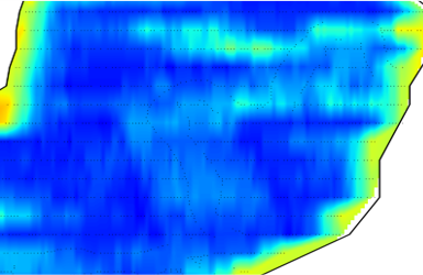
In-Depth's patented Mutual Coherency Maps give a visual QC of the survey design, mathematically predicting reconstruction quality based on the local arrangement of nodes around every point in the survey.
For some background on MC Maps, check out this blog article: Compressive Seismic - Survey Design QC
Step 5 - Iterate
It is normal for there to be some interactive changes at this point as obstacles are updated. It is even possible to change the initial pre-plot at this stage. The CSA program can be re-run as many times as necessary to converge on the final design.
Step 6 - Acquisition

With a finalized design, it is time to select an acquisition contractor and get the data acquired. Should the obstacles change during acquisition, the CS design will be re-calculated and updated for any locations that were not yet acquired.
Step 7 - Processing & Reconstruction

There will be at least two passes of reconstruction applied in processing: a raw reconstruction (generally for archive purposes) and a final reconstruction just before migration when the noise and statics issues have been addressed. It is possible to reconstruct at any stage—for example, after ground roll removal—to achieve a better result. Here's a closer look at reconstruction in an earlier blog post: Compressive Seismic - Is it interpolation?
Conclusion
Compressive Seismic is a game-changer for seismic data. It can either reduce your acquisition cost or increase your data quality with a simple change to the layout of the survey pattern.
The reward is certainly worth the few extra steps.
Check out the publication tab at the top of the page for additional information on patents, technical papers and presentations.
